Creating Arrays
In the previous section, we looked at NumPy’s basic data structure for representing arrays, the ndarray class, and we looked at the basic attributes of this class. In this section we focus on functions from the NumPy library that can be used to create ndarray instances.
NumPy provides a set of functions generate ndarrays depending on their properties and the applications they are used for. Throughout this tutorial you’ll discover that these features will be useful.
Arrays Created from Lists and Other Array-like Objects
- Using the
np.array()function, NumPy arrays can be constructed from explicit Python lists, iterable expressions and other array-like objects (such as otherndarrayinstances).
import numpy as np
%matplotlib inline
import matplotlib.pyplot as plt
data = np.array([1, 3, 9]) # Create a one-dimensional array from a Python list
data
data.ndim
data.shape
data = np.array([[1, 2], [5, 7]]) # Create 2D array using nested Python lists
data
data.ndim
data.shape
Arrays Filled with Constant Values
- The functions
np.zeros()andnp.ones()create and return arrays filled with zeros and ones respectively. - They take, as first argument, an integer or a tuple that describes the number of elements along each dimension of the array
np.zeros((2, 3))
np.ones(5)
- Like other array-generating functions, these functions also accept an optional keyword argument that specifies the data type for the elements in the array.
- By default, the data type is
float64:
data = np.ones(10)
data
data.dtype
data = np.ones(5, dtype=complex)
data
data.dtype
- Arrays filled with an arbitrary constant value can be generated by first creating an array filled with ones and then multiplying the array with the desired fill value.
- However, NumPy also provides the function
np.full()that does exactly this in one step:
x = 10.5 * np.ones(5)
x
y = np.full(shape=5, fill_value=10.5)
y
- An already created array can also be filled with constant values using the
np.fill()function, which takes an array and a value as arguments, and set all elements in the array to the given value:
x1 = np.empty(3) # generates an array with uninitialized values, of the given size
x1
x1.fill(np.pi)
x1
Arrays Filled with Logarithmic Sequences
The function np.logspace() is similar to np.linspace(), but the increments between the elements in the array are logarithmically distributed, and the first two arguments, for the start and end values, are the powers of the optional base keyword argument (which defaults to 10):
# Generate 5 points between 10**0= 1 and 10**2=100
np.logspace(start=0, stop=2, num=5)
Meshgrid Arrays
- Multidimensional coordinate grids can be generated using the function
np.meshgrid(). - Given two one-dimensional coordinate arrays, we can generate two-dimensional coordinate arrays using the
np.meshgrid()function:
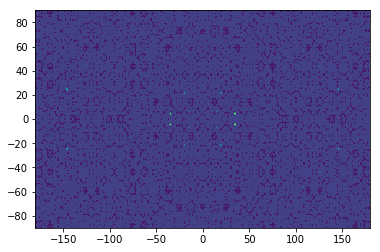
# 1-D arrays representing the coordinates of a grid
y = np.linspace(-90., 90., num=180)
x = np.linspace(-180., 180., 360)
xc, yc = np.meshgrid(x, y)
z = np.sin(xc**2 + yc**2) / np.cos(xc**2 + yc**2)
xc
yc
z
plt.contourf(x, y, z)
- It is also possible to generate higher-dimensional coordinate arrays by passing
more arrays as argument to the
np.meshgrid()function
Creating Uninitialized Arrays
-
To create an array of specific size and data type, but without initializing the elements of the array to any particular values, we can use the function
np.empty() -
The advantage of this function, for example, instead of
np.zeros, is that we can avoid the initiation step. If all elements are guaranteed to be initialized later in the code, this can save a little bit of time, especially when working with large arrays:
np.empty(shape=5, dtype=np.float64)
NOTE:
- There’s no guarantee that elements generated by
np.empty()have any particular values. For this reason it is important that all values are explicitly assigned before the array is used; otherwise unpredictable errors are likely to arise.
Creating Arrays with Properties of Other Arrays
It is often necessary to create new arrays that share properties, such as shape and data type with another array. NumPy provides a family of functions for this purpose:
np.ones_like()np.zeros_like()np.full_like()np.empty_like()
A typical use-case is a function that takes arrays of unspecified type and size as arguments and requires working with arrays of the same size and type.
data = np.array([[2, 3, 8], [6, 8, 10]], dtype=np.float32)
data
np.ones_like(data)
np.zeros_like(data)
fill_value = np.sin(np.deg2rad(90))
np.full_like(data, fill_value=fill_value)
Creating Matrix Arrays
NumPy provides functions for generating commonly used matrixes. One of these functions is np.identity() which generates a square matrix with oens on the diagonal and zeros elsewhere:
np.identity(6)
The similar function np.eye() generates matrices with ones on a diagonal (optionally offset):
np.eye(N=4, M=5, k=1)
where:
- N: is the number of rows in the output
- M: is the number of columns in the output
- k: Index of the diagonal: 0 (the default) refers to the main diagonal, a positive value refers to an upper diagonal, and a negative value to a lower diagonal.a
np.eye(N=4, M=5, k=-1)
To construct a matrix with an arbitrary one-dimensional array on the diagonal, we can use the np.diag() function (which also takes the optional keyword argument k to specify an offset from the diagonal) :
d = np.arange(0, 20, 4)
d
np.diag(v=d, k=0)
np.diag(v=d, k=-1)
%load_ext watermark
%watermark --iversion -g -m -v -u -d